ツール紹介ページ

はじめに

免責事項

本文書はDS2022データセットを利用しようと考えている方向けに提供している情報です。しかし、本文書を利用して生じるいかなる損害についても、責任は負いません。利用者の責任での利用をお願いします。

前書き

気候予測データセット2022の主要なファイル・フォーマットやその描画ツール等について、サンプルデータを用いて解説する。ツール類のインストール等については、環境構築を参照されたい。なお、サンプルデータには、参考資料の充実度を考慮し、必要に応じて気候予測データ以外のデータを用いる。

DS2022気候予測データの主要なファイル・フォーマット

GRIB / GRIB2

世界気象機関（WMO）で策定したフォーマットであり、数値気象予報モデルの出力であるグリッドデータを各国の気象現業機関の間で交換することなどに使用されている。 GRIBは気象庁55年長期再解析（JRA-55）でも使用されている第1版と、現行の第2版（GRIB2）の二つの版が広く利用されている。なお、以降の解説では、区別のため第1版についてはGRIB1と表記する場合がある。座標系や各種パラメータが格納されており、ファイルサイズを小さくするためにデータの圧縮が行われる。そのため同じデータをGRIB1/GRIB2と後述するNetCDFファイルに格納した場合では、GRIB1/GRIB2のファイルサイズが小さいことが多い。またデータファイルに格納されている変数の名前や単位は、パラメータについてのテーブル（parameter table）を参照する形となっている。例えば「 JRA-55プロダクト利用手引書 1.25度緯度／経度格子データ編」の等圧面解析値(anl_p125)の出力要素の表4-5を見たとき、表の一番左のカラムの「数字符号」に対応するパラメータ（変数名）と単位がその右側に書かれている。

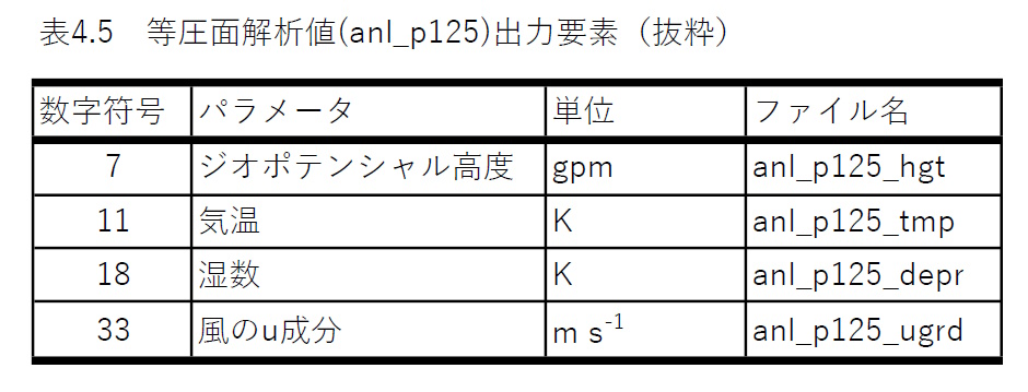
表1. JRA-55 表4.5の抜粋

このような情報をそれぞれのツールのparameter tableのフォーマットに従ってテキストファイルに書き出しておく必要がある。

NetCDF

米国のUniversity Corporation of Atmospheric Research (UCAR) の Unidata プログラムで開発されたデータフォーマット。「世界気候研究計画(WCRP)」のもとで実施されている「結合モデル相互比較プロジェクト(CMIP)」に提出される気候モデルのデータはこのNetCDF形式のフォーマットに格納したものである。データファイルは、ヘッダー部（格子の情報などを含む）とデータ部からなる。ファイルの中には格子やデータ自体に関する属性も格納されており、データファイルを読むだけで、どのようなデータがファイルに格納されているのかを理解できる（自己記述式）。通常は4バイト実数でデータを格納するが、そのままではファイルサイズが大きくなることが多く、過去に用いられていたコンピューターのファイルシステムではデータを格納できないことがあった（例えばFAT32では1ファイルの容量は最大4GBであった）。そのため”y = ix * scale + offset”という変換式を利用して符号付き2バイト整数（short int）で格納してファイルサイズを小さくすることがあった（例えば1990年代後半に公開されたNCEP-NCAR大気再解析データ）。なお、最新のNetCDF4ライブラリでは圧縮ライブラリを用いてファイルサイズを小さくすることができるようになっている。

いわゆる「GrADS形式」

次の枠の中のコード片のようにFortranでunformattedかつdirectで書き出したバイナリファイル（時にはsequentialで書き出したものもある）。


real varray(ix, iy)
open(10, file=’tmp.bin’, form=’unformatted’, access=’direct’, recl=ix*iy*4)
write(10, rec=1) varray

通常は4バイト（32ビット）の実数（float）で書き出す。一方、ファイルサイズを小さくするために、“y = ix * scale + offset”という変換式を利用して、2バイト符号あり整数（short int）に変換して書き出すこともある。 GrADSでは4バイト実数で格納されたファイルも2バイト符号あり整数で格納されたファイルも読み込むことができる。またデータファイル自身にはデータが格納されているのみであり、「どのような変数がどのような次元をもっているのか」などの情報は別途コントロールファイルとして提供される。特に、データが北から南に向けて格納されているのか、データがlittle endianで書き出されたものなのかそれともbig endianで書き出されたのかといった情報もコントロールファイルに含まれている。

サンプルデータ

本文書で使用するサンプルデータを列挙する。それぞれの公開先からダウンロードをすること。

NOAA Extended Reconstructed SST V5

米国 NOAA Physical Sciences Laboratory から公開されている海面水温データ “NOAA Extended Reconstructed SST V5 (ERSST)”をダウンロードする。


$ wget https://downloads.psl.noaa.gov/Datasets/noaa.ersst.v5/sst.mnmean.nc

# ファイルに含まれているデータの情報を確認。
$ ncdump -h sst.mnmean.nc
netcdf sst.mnmean {
dimensions:
        lat = 89 ;
        lon = 180 ;
        time = UNLIMITED ; // (2026 currently)
        nbnds = 2 ;
variables:
        float lat(lat) ;
                lat:units = "degrees_north" ;
                lat:long_name = "Latitude" ;
                lat:actual_range = 88.f, -88.f ;
                lat:standard_name = "latitude" ;
                lat:axis = "Y" ;
                lat:coordinate_defines = "center" ;
        float lon(lon) ;
                lon:units = "degrees_east" ;
                lon:long_name = "Longitude" ;
                lon:actual_range = 0.f, 358.f ;
                lon:standard_name = "longitude" ;
                lon:axis = "X" ;
                lon:coordinate_defines = "center" ;
        double time_bnds(time, nbnds) ;
                time_bnds:long_name = "Time Boundaries" ;
        double time(time) ;
                time:units = "days since 1800-1-1 00:00:00" ;
                time:long_name = "Time" ;
                time:delta_t = "0000-01-00 00:00:00" ;
                time:avg_period = "0000-01-00 00:00:00" ;
                time:prev_avg_period = "0000-00-07 00:00:00" ;
                time:standard_name = "time" ;
                time:axis = "T" ;
                time:actual_range = 19723., 81357. ;
        float sst(time, lat, lon) ;
                sst:long_name = "Monthly Means of Sea Surface Temperature" ;
                sst:units = "degC" ;
                sst:var_desc = "Sea Surface Temperature" ;
                sst:level_desc = "Surface" ;
                sst:statistic = "Mean" ;
                sst:missing_value = -9.96921e+36f ;
                sst:dataset = "NOAA Extended Reconstructed SST V5" ;
                sst:parent_stat = "Individual Values" ;
                sst:actual_range = -1.8f, 42.32636f ;
                sst:valid_range = -1.8f, 45.f ;
// global attributes:
<<以下省略>>

変数としてlat, lon, time_bnds, time, sstが含まれている。このうちlat, lon, timeは次元を表現する1次元データであり、海面水温sstはsst(time, lat, lon)と表示されており、経度・緯度・時間の3次元データであることがわかる。また、sst:long_name = “Monthly Means of Sea Surface Temperature”や sst:units = “degC”などは変数sstの属性である。 NetCDFでは属性を適切に付与することにより、どのようなデータがこのファイルに格納されているのかを知ることができるようになっている。

気象庁55年長期再解析(JRA-55)

DIASから公開されている気象庁55年長期再解析（JRA-55）のうち、anl_surf125の気候値（/jra55/Clim9120/Monthly/anl_surf125）のデータをダウンロードする。そして、拡張子が”.ctl”となっているコントロールファイルと”.idx”となっているインデックスファイルも入手する。また、anl_surf125の月別データ(/jra55/Hist/Monthly/anl_surf125)の2022年1月のデータを入手する。

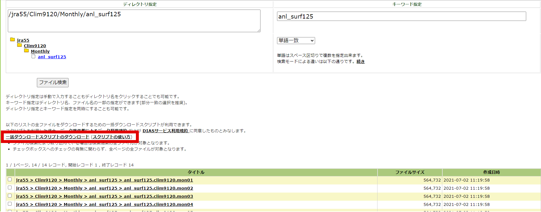
図1. DIASでのJRA-55 anl_surf125検索画面


# 上の赤枠のところに表示されている【一括ダウンロードスクリプト】を利用する際
# Python2が必要となる。condaで

$ conda create -n py27 python=2.7

# として、Python 2.7が動く仮想環境を作成しておく。
# 仮想環境py27をアクティベートして、
# 一括ダウンロードスクリプトを用いてデータをダウンロードする。
# UsernameにはDIASのアカウントを、PasswordにはDIASのパスワードを入力する。

$ conda activate py27
$ python2 ./download.py
Username:abcd1234@example.com
Password:xxxxxxxxxxx

# ダウンロード終了後にconda環境を終了する。
$ conda deactivate

d4PDF_RCM

気候予測データセット2022の「全球及び日本域確率的気候予測データ（d4PDFシリーズ）」の日本域ダウンスケーリングデータである d4PDF_RCMの過去実験(HPB)のアンサンブルメンバーm001の2000年1月の地上大気データと実験共通の標高分布・海陸分布データをダウンロードする。 d4PDFのダウンロードは「d4PDFダウンロード」から実行できる。

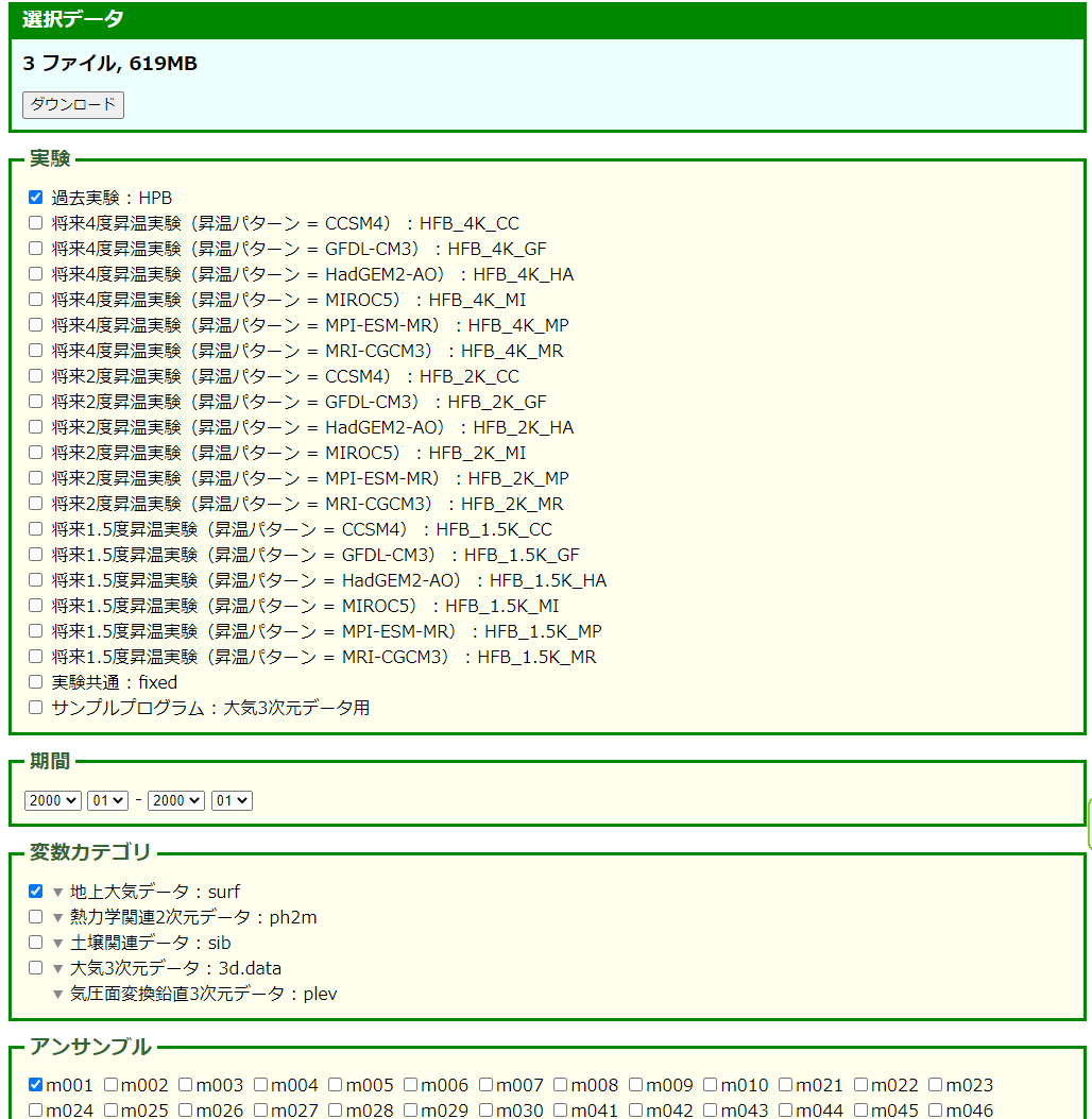
図2. DIASでのd4PDF_RCMの地上要素検索画面

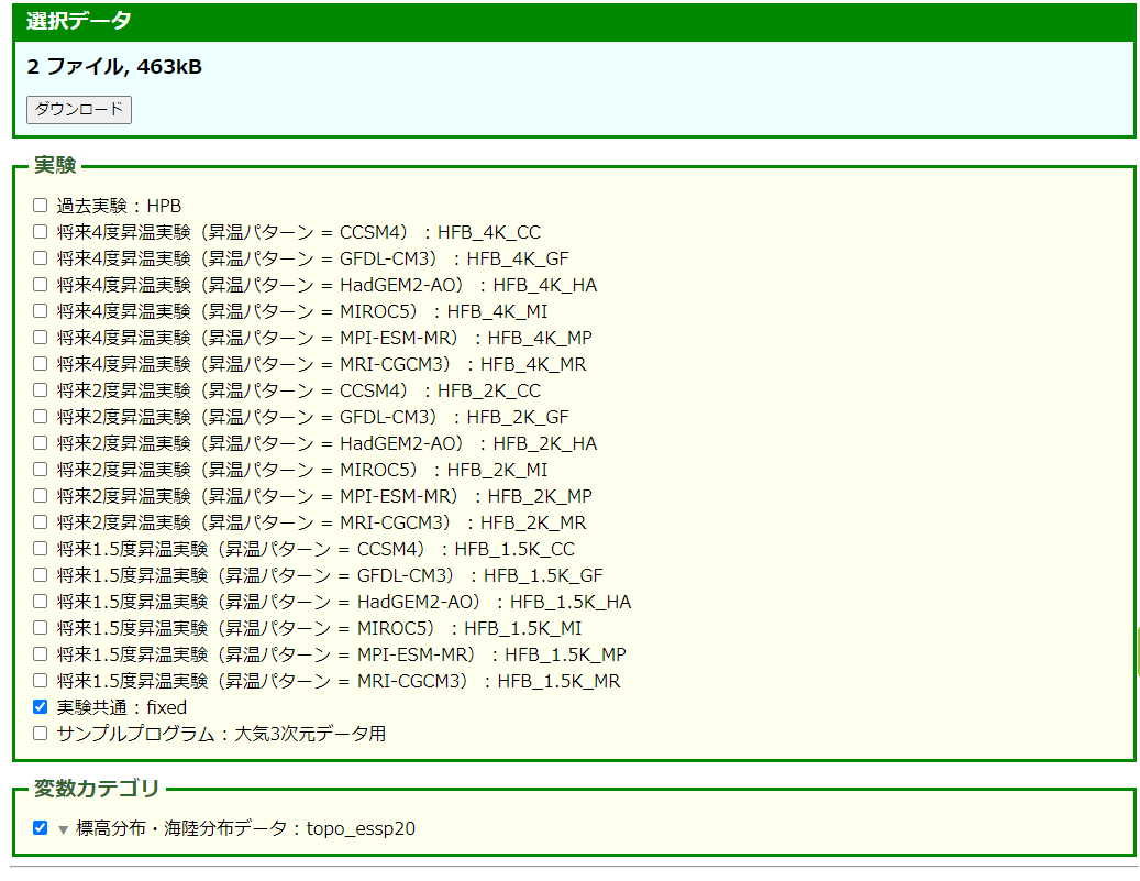
図3. DIASでのd4PDF_RCMのfixedデータ検索画面

まずは2000年1月のデータをダウンロードする。 files.tar という名前でダウンロードされるので、ダウンロードしたら


$ tar xvf files.tar

として解凍する。その後は


$ mv files.tar files.surf20001.tar

のように改名しておく。同様に標高分布・海陸分布データをダウンロードし解凍する。

過去実験データは d4PDF_RCM/HPB/m001/1999 以下に


surf_HPB_m001_200001.ctl, surf_HPB_m001_200001.grib, surf_HPB_m001_200001.idx

が書き出される。標高分布・海陸分布データは d4PDF_RCM/fixed 以下に


topo_essp20.ctl, topo_essp20.dat

が書き出される。

GrADSのexampleデータ

米国 George Mason University の The Center for Ocean-Land-Atmosphere Studies の GrADS のウェブページにある example.tar.gz をダウンロードする。


$ wget ftp://cola.gmu.edu/grads/example.tar.gz
$ tar zxvf example.tar.gz
model.ctl  model.dat  tutorial

データ・ビューアー

ncview

米国 Scripps Institution of Oceanography の Pierce 氏が作成したNetCDF形式ファイル用のデータ・ビューアー。

ターミナルの中で以下のようにして起動。


$ ncview sst.mnmean.nc

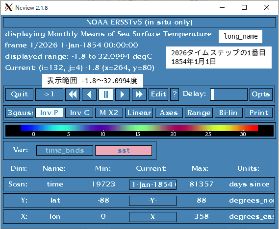
図4. ncview のメイン画面

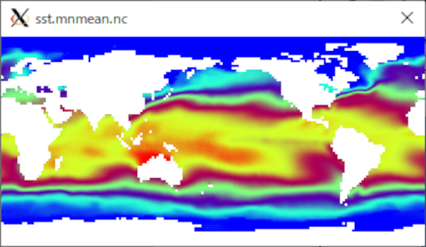
図5. ncview のデータ表示画面

Panoply

米国 NASA Goddard Institute for Space Studiesで開発されたデータ・ビューアー。 NetCDF / HDF / GRIB形式ファイルの可視化に利用できる。


$ panoply.sh

として、起動。ファイル選択画面からファイルを選択。

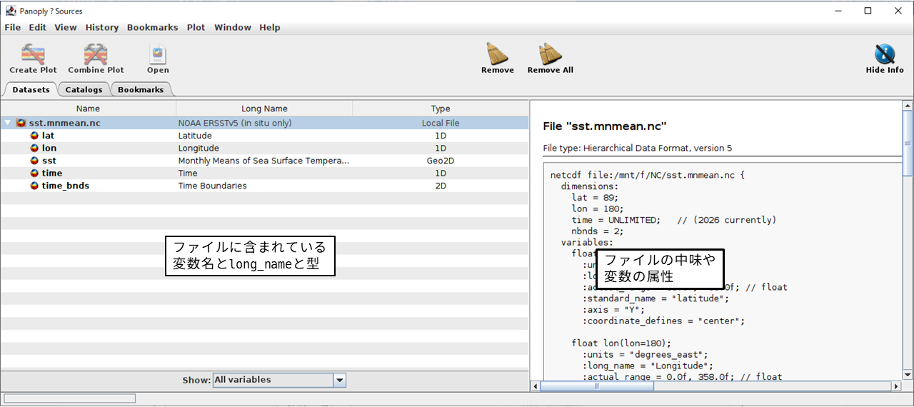
図6. Panoplyのメイン画面

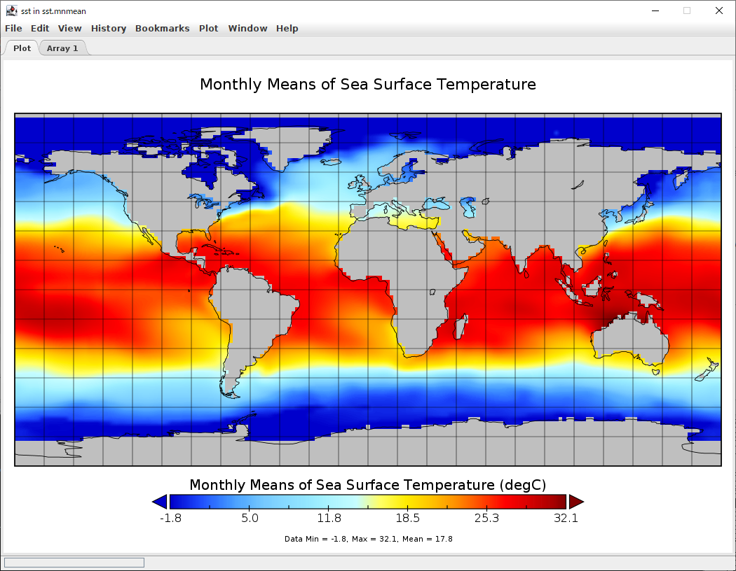
図7. Panoplyで描画した画面

wgrib / wgrib2

米国のNOAA Climate Prediction Centerから公開されている。

wgrib : GRIBのデータを処理するときに使用する。
wgrib2 : GRIB2のデータを処理するときに使用する。
【参考】日本自動車研究所の早崎氏が公開されているwgrib/wgrib2の使い方の情報のページ。
- wgrib使用方法
- wgrib2使用方法

パラメータテーブル

wgrib / wgrib2に内蔵されていないGRIBのパラメータテーブルを使用しているデータを読む際には、ユーザーがパラメータテーブルを用意する必要がある。 JRA-55の場合、「JRA-55プロダクト利用手引書」を参照すればよい。または、GrADS用のコントロールファイルがあれば、そこから数字符号を入手することもできる。

JRA-55のパラメータテーブルを作成し、エクスポートする。


$ less JRA55_anl_surf_ptable_wgrib.txt
-1:34:241:200
1:pres:"surface pressure [Pa]"
2:msl:"mean sea level pressure [Pa]"
11:airt:"air temperature [K]"
13:pott:"potential temperature [K]"
18:depr:"dewpoint depression [K]"
51:sphum:"speciphic humidity [kg/kg]"
52:rhum:"relative humidity [%]"
33:uwnd:"eastward wind [m/s]"
34:vwnd:"northward wind [m/s]"

$ export GRIBTAB=./JRA55_anl_surf_ptable_wgrib.txt

ファイルの確認

JRA-55のanl_surf125 の平年値ファイルの中味を確認する。

$ wgrib anl_surf125.clim9120.mon01
1:0:d=91010100:pres:kpds5=1:kpds6=1:kpds7=0:TR=51:P1=0:P2=1:TimeU=3:sfc:0-1mon product:ave@1yr:NAve=30
2:62748:d=91010100:pott:kpds5=13:kpds6=1:kpds7=0:TR=51:P1=0:P2=1:TimeU=3:sfc:0-1mon product:ave@1yr:NAve=30
3:125496:d=91010100:msl:kpds5=2:kpds6=102:kpds7=0:TR=51:P1=0:P2=1:TimeU=3:MSL:0-1mon product:ave@1yr:NAve=30
4:188244:d=91010100:airt:kpds5=11:kpds6=105:kpds7=2:TR=51:P1=0:P2=1:TimeU=3:2 m above gnd:0-1mon product:ave@1yr:NAve=30
5:250992:d=91010100:depr:kpds5=18:kpds6=105:kpds7=2:TR=51:P1=0:P2=1:TimeU=3:2 m above gnd:0-1mon product:ave@1yr:NAve=30
6:313740:d=91010100:sphum:kpds5=51:kpds6=105:kpds7=2:TR=51:P1=0:P2=1:TimeU=3:2 m above gnd:0-1mon product:ave@1yr:NAve=30
7:376488:d=91010100:rhum:kpds5=52:kpds6=105:kpds7=2:TR=51:P1=0:P2=1:TimeU=3:2 m above gnd:0-1mon product:ave@1yr:NAve=30
8:439236:d=91010100:uwnd:kpds5=33:kpds6=105:kpds7=10:TR=51:P1=0:P2=1:TimeU=3:10 m above gnd:0-1mon product:ave@1yr:NAve=30
9:501984:d=91010100:vwnd:kpds5=34:kpds6=105:kpds7=10:TR=51:P1=0:P2=1:TimeU=3:10 m above gnd:0-1mon product:ave@1yr:NAve=30

Unix環境ではwgrib/wgrib2とcatやgrepなどの併用で、データの追加または抽出ができる。また、GRIB形式のファイルからGrADSで用いられるバイナリファイルに変換することができる。

データの抽出

anl_surf125の平年値ファイルから気圧データだけを抽出し、バイナリファイルに変換する。なお”\“は継続行を意味する。


$ wgrib anl_surf125.clim9120.mon01 | grep “:pres:” |  \
wgrib anl_surf125.clim9120.mon01 -i -bin -nh \
-o anl_surf125.clim9120.mon01.pres.bin

Climate Data Operators (cdo)

ドイツのMax-Planck-Institut fur Meteorologie から公開されている。 NetCDF形式、GRIB形式、GrADS形式のファイルの操作をすることができるツールである。

パラメータテーブル

cdoに含まれていないGRIBのパラメータテーブルを用いたファイルをcdoで処理する際には、ユーザーがパラメータテーブルを作成する必要がある。 JRA-55の場合、「JRA-55プロダクト利用手引書」を参照すればよい。または、GrADS用のコントロールファイルがあれば、そこから数字符号を入手することもできる。


$ less JRA55_anl_surf_ptable_cdo.txt
1   pres   pressure　　[Pa]
2   msl    mean sea level pressure [Pa]
11  airt   air temperature　 [K]
13  pott   potential temperature   [K]
18  depr   dewpoint depression     [K]
51  sphum  speciphic humidity      [kg/kg]
52  rhum   relative humidity       [%]
33  uwnd   eastward wind　   [m/s]
34  vwnd   northward wind　  [m/s]
$

ファイルの確認

パラメータテーブルを"-t"のオプションで指定して、ファイルの中味を確認する。


# ファイルの中味の確認。
# JRA-55のファイルの時間平均のパラメータが理解できないとエラーが出力されるが、データは読むことができる。
$ cdo -t JRA55_anl_surf_ptable_cdo.txt infon anl_surf125.clim9120.mon01
ECCODES ERROR   :  Unknown stepType=[51] timeRangeIndicator=[51]
<<エラー中略>>
-1 :       Date     Time   Level Gridsize    Miss :     Minimum　Mean     Maximum : Parameter name
1 : 1991-01-01 00:00:00       0    41760       0 :      51862.      96635.  1.0284e+05 : pres
2 : 1991-01-01 00:00:00       0    41760       0 :      239.76      280.06      323.57 : pott
3 : 1991-01-01 00:00:00       0    41760       0 :      98292.  1.0101e+05  1.0417e+05 : msl
4 : 1991-01-01 00:00:00       2    41760       0 :      239.19      277.04      306.51 : airt
5 : 1991-01-01 00:00:00       2    41760       0 :     0.80086      3.5672      26.121 : depr
6 : 1991-01-01 00:00:00       2    41760       0 :  0.00014653   0.0072782    0.020822 : sphum
7 : 1991-01-01 00:00:00       2    41760       0 :      18.014      79.283      92.421 : rhum
8 : 1991-01-01 00:00:00      10    41760       0 :     -10.454   -0.060975      9.4525 : uwnd
9 : 1991-01-01 00:00:00      10    41760       0 :     -9.5364    -0.20628      9.3699 : vwnd
cdo    infon: Processed 375840 values from 9 variables over 1 timestep [0.06s 47MB].

GRIB1形式からNetCDF形式への変換

GRIB1形式であるJRA-55のデータをNetCDF形式に変換する。 "-f nc copy" で変換できる。


$ cdo -t JRA55_anl_surf_ptable_cdo.txt -f nc copy anl_surf125.clim9120.mon01 anl_surf125.clim9120.mon01.nc
ECCODES ERROR   :  Unknown stepType=[51] timeRangeIndicator=[51]
<<エラー中略>>
cdo    copy: Processed 375840 values from 9 variables over 1 timestep [0.15s 51MB].

GrADS用バイナリファイルからNetCDF形式への変換

GrADS用バイナリファイルをNetCDF形式に変換するには"-f nc import_binary"を用いる。なおバイナリファイナル自身ではなく、コントロールファイルを引数として与える。


$ cdo -f nc import_binary model.ctl model.nc
cdo    import_binary: Processed 8 variables [0.22s 44MB].
$ cdo sinfon model.nc
   File format : NetCDF2
    -1 : Institut Source   T Steptype Levels Num    Points Num Dtype : Parameter name
     1 : unknown  unknown  v instant       1   1      3312   1  F32  : ps
     2 : unknown  unknown  v instant       7   2      3312   1  F32  : u
     3 : unknown  unknown  v instant       7   2      3312   1  F32  : v
     4 : unknown  unknown  v instant       7   2      3312   1  F32  : hgt
     5 : unknown  unknown  v instant       7   2      3312   1  F32  : tair
     6 : unknown  unknown  v instant       5   3      3312   1  F32  : q
     7 : unknown  unknown  v instant       1   1      3312   1  F32  : tsfc
     8 : unknown  unknown  v instant       1   1      3312   1  F32  : p
   Grid coordinates :
     1 : lonlat                   : points=3312 (72x46)
                              lon : 0 to 355 by 5 degrees_east  circular
                              lat : -90 to 90 by 4 degrees_north
   Vertical coordinates :
     1 : surface                  : levels=1
     2 : generic                  : levels=7
                              lev : 1000 to 100
     3 : generic                  : levels=5
                            lev_2 : 1000 to 300
   Time coordinate :
                             time : 5 steps
     RefTime =  1987-01-02 00:00:00  Units = hours  Calendar = standard
  YYYY-MM-DD hh:mm:ss  YYYY-MM-DD hh:mm:ss  YYYY-MM-DD hh:mm:ss  YYYY-MM-DD hh:mm:ss
  1987-01-02 00:00:00  1987-01-03 00:00:00  1987-01-04 00:00:00  1987-01-05 00:00:00
  1987-01-06 00:00:00
cdo    sinfon: Processed 8 variables over 5 timesteps [0.01s 45MB].

指定した変数の抽出

複数の変数が格納されているファイルから指定した変数だけを抽出する。


# 地上気圧データを抽出する。
$ cdo select,name=ps model.nc ps.nc

# 気温データを抽出する。
$ cdo select,name=tair model.nc tair.nc

指定した年のデータの抽出

NetCDF形式のERSSTのデータファイルから指定した年のデータを抽出する。


# 1991年の海面水温データを抽出する。
$ cdo select,year=1991/1991/1 sst.mnmean.nc sst.1991.nc

# ファイルの中味の確認。
$ cdo sinfo sst.1991.nc
   File format : NetCDF4 classic
    -1 : Institut Source   T Steptype Levels Num    Points Num Dtype : Parameter ID
     1 : unknown  In situ  v instant       1   1         2   1  F64  : -1
     2 : unknown  In situ  v instant       1   1     16020   2  F32  : -2
   Grid coordinates :
     1 : generic                  : points=2
     2 : lonlat                   : points=16020 (180x89)
                              lon : 0 to 358 by 2 degrees_east  circular
                              lat : 88 to -88 by -2 degrees_north
   Vertical coordinates :
     1 : surface                  : levels=1
   Time coordinate :
                             time : 12 steps
     RefTime =  1800-01-01 00:00:00  Units = days  Calendar = standard
  YYYY-MM-DD hh:mm:ss  YYYY-MM-DD hh:mm:ss  YYYY-MM-DD hh:mm:ss  YYYY-MM-DD hh:mm:ss
  1991-01-01 00:00:00  1991-02-01 00:00:00  1991-03-01 00:00:00  1991-04-01 00:00:00
  1991-05-01 00:00:00  1991-06-01 00:00:00  1991-07-01 00:00:00  1991-08-01 00:00:00
  1991-09-01 00:00:00  1991-10-01 00:00:00  1991-11-01 00:00:00  1991-12-01 00:00:00
cdo    sinfo: Processed 2 variables over 12 timesteps [0.02s 45MB].

1991年の各月の月初の時刻が表示され、1991年の12個のデータが抽出されたことがわかる。

同様にして、1992年のデータだけを格納しているファイルと、1993年のデータだけを格納しているファイルを作成する。

$ cdo select,year=1992/1992/1 sst.mnmean.nc sst.1992.nc
$ cdo select,year=1993/1993/1 sst.mnmean.nc sst.1993.nc

ファイルの結合

緯度・経度・高さ/深さの各次元の格子数が同一である年別のデータファイルを"mergetime"を用いて結合できる。1991年、1992年、1993年の海面水温データを一つのファイルに結合する。


$ cdo mergetime sst.1991.nc sst.1992.nc sst.1993.nc sst.1991-1993.nc
cdo    mergetime: Processed 576792 values from 6 variables over 36 timesteps [0.17s 51MB].

ファイルの中味の確認。


$ cdo sinfo sst.1991-1993.nc
   File format : NetCDF4 classic
    -1 : Institut Source   T Steptype Levels Num    Points Num Dtype : Parameter ID
     1 : unknown  In situ  v instant       1   1         2   1  F64  : -1
     2 : unknown  In situ  v instant       1   1     16020   2  F32  : -2
   Grid coordinates :
     1 : generic                  : points=2
     2 : lonlat                   : points=16020 (180x89)
                              lon : 0 to 358 by 2 degrees_east  circular
                              lat : 88 to -88 by -2 degrees_north
   Vertical coordinates :
     1 : surface                  : levels=1
   Time coordinate :
                             time : 36 steps
     RefTime =  1800-01-01 00:00:00  Units = days  Calendar = standard
  YYYY-MM-DD hh:mm:ss  YYYY-MM-DD hh:mm:ss  YYYY-MM-DD hh:mm:ss  YYYY-MM-DD hh:mm:ss
  1991-01-01 00:00:00  1991-02-01 00:00:00  1991-03-01 00:00:00  1991-04-01 00:00:00
  1991-05-01 00:00:00  1991-06-01 00:00:00  1991-07-01 00:00:00  1991-08-01 00:00:00
  1991-09-01 00:00:00  1991-10-01 00:00:00  1991-11-01 00:00:00  1991-12-01 00:00:00
  1992-01-01 00:00:00  1992-02-01 00:00:00  1992-03-01 00:00:00  1992-04-01 00:00:00
  1992-05-01 00:00:00  1992-06-01 00:00:00  1992-07-01 00:00:00  1992-08-01 00:00:00
  1992-09-01 00:00:00  1992-10-01 00:00:00  1992-11-01 00:00:00  1992-12-01 00:00:00
  1993-01-01 00:00:00  1993-02-01 00:00:00  1993-03-01 00:00:00  1993-04-01 00:00:00
  1993-05-01 00:00:00  1993-06-01 00:00:00  1993-07-01 00:00:00  1993-08-01 00:00:00
  1993-09-01 00:00:00  1993-10-01 00:00:00  1993-11-01 00:00:00  1993-12-01 00:00:00
cdo    sinfo: Processed 2 variables over 36 timesteps [0.02s 45MB].

指定した領域のデータの切り出し

領域を指定してデータを切り出す。次の例は、東経120度から東経180度、北緯20度から北緯50度の領域の海面水温データを切り出す。


$ cdo sellonlatbox,120,180,20,50 sst.1991.nc sst.1991.sub.nc
$ cdo sinfo sst.1991.sub.nc
   File format : NetCDF4 classic
    -1 : Institut Source   T Steptype Levels Num    Points Num Dtype : Parameter ID
     1 : unknown  In situ  v instant       1   1         2   1  F64  : -1
     2 : unknown  In situ  v instant       1   1       496   2  F32  : -2
   Grid coordinates :
     1 : generic                  : points=2
     2 : lonlat                   : points=496 (31x16)
                              lon : 120 to 180 by 2 degrees_east
                              lat : 50 to 20 by -2 degrees_north
   Vertical coordinates :
     1 : surface                  : levels=1
   Time coordinate :
                             time : 12 steps
     RefTime =  1800-01-01 00:00:00  Units = days  Calendar = standard
  YYYY-MM-DD hh:mm:ss  YYYY-MM-DD hh:mm:ss  YYYY-MM-DD hh:mm:ss  YYYY-MM-DD hh:mm:ss
  1991-01-01 00:00:00  1991-02-01 00:00:00  1991-03-01 00:00:00  1991-04-01 00:00:00
  1991-05-01 00:00:00  1991-06-01 00:00:00  1991-07-01 00:00:00  1991-08-01 00:00:00
  1991-09-01 00:00:00  1991-10-01 00:00:00  1991-11-01 00:00:00  1991-12-01 00:00:00
cdo    sinfo: Processed 2 variables over 12 timesteps [0.02s 46MB].

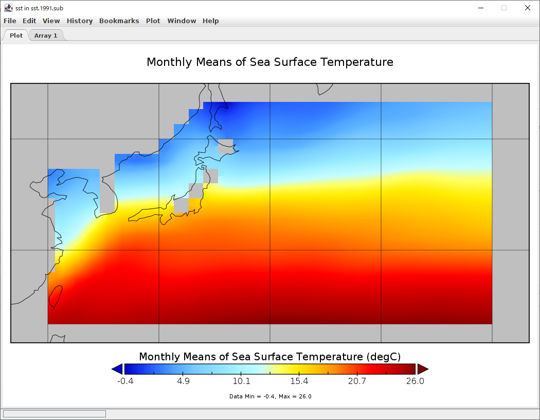
図8. 日本付近のERSST切り出し

panoplyで表示すると上のように日本付近が切り出されていることがわかる。

統計値の作成

月平均値から各年の年平均値を作成。


$ cdo yearmonmean sst.1991-1993.nc sst.1991-1993.yearmean.nc
$ cdo sinfo sst.1991-1993.yearmean.nc
   File format : NetCDF4 classic
    -1 : Institut Source   T Steptype Levels Num    Points Num Dtype : Parameter ID
     1 : unknown  In situ  v instant       1   1         2   1  F64  : -1
     2 : unknown  In situ  v instant       1   1     16020   2  F32  : -2
   Grid coordinates :
     1 : generic                  : points=2
     2 : lonlat                   : points=16020 (180x89)
                              lon : 0 to 358 by 2 degrees_east  circular
                              lat : 88 to -88 by -2 degrees_north
   Vertical coordinates :
     1 : surface                  : levels=1
   Time coordinate :
                             time : 3 steps
     RefTime =  1800-01-01 00:00:00  Units = days  Calendar = standard  Bounds = true
  YYYY-MM-DD hh:mm:ss  YYYY-MM-DD hh:mm:ss  YYYY-MM-DD hh:mm:ss  YYYY-MM-DD hh:mm:ss
  1991-06-16 00:00:00  1992-06-16 00:00:00  1993-06-16 00:00:00
cdo    sinfo: Processed 2 variables over 3 timesteps [0.02s 46MB].

$ ncview sst.1991-1993.yearmean.nc

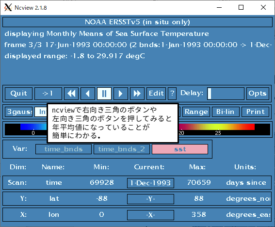
図9. ncviewで時間を確認する

GrADS

米国 George Mason University の The Center for Ocean-Land-Atmosphere Studiesで開発されたソフトウェア。
バイナリファイルは, コントロールファイルを”open test.ctl”として読み込む。
NetCDFファイル（COARDS convention / CF convention）を”sdfopen test.nc”として読み込む。
読み込むことができないNetCDFファイルは、コントロールファイルを作成して、xdfopenコマンドを利用してデータを読み込む。
GRIBのファイルは “grib2ctl.pl”、 GRIB2のファイルは “g2ctl” を用いてコントロールファイルを作成し、gribmapでインデックスファイルを作成することによりGrADSでGRIBデータを読み込むことができる。
公式チュートリアル（英文）
【参考】東北大学大学院気象学・大気力学分野が公開されている「GrADSのTips」
【参考】筑波大学生命環境系の釜江陽一氏が公開されている「GrADS-Note」

GrADS用バイナリファイルmodel.datを読む

GrADSのチュートリアルに用いられる”model.dat”を読む。


$ grads
Grid Analysis and Display System (GrADS) Version 2.2.1
Copyright (C) 1988-2018 by George Mason University
GrADS comes with ABSOLUTELY NO WARRANTY
See file COPYRIGHT for more information

Config: v2.2.1 little-endian readline grib2 netcdf hdf4-sds hdf5 opendap-grids,stn geotiff shapefile
Issue 'q config' and 'q gxconfig' commands for more detailed configuration information
Landscape mode? ('n' for portrait):
GX Package Initialization: Size = 11 8.5
ga-> open model.ctl
Scanning description file:  model.ctl
Data file model.dat is open as file 1
LON set to 0 360
LAT set to -90 90
LEV set to 1000 1000
Time values set: 1987:1:2:0 1987:1:2:0
E set to 1 1

# ファイルの中味を確認。
ga -> q file 1
File 1 : 5 Days of Sample Model Output
  Descriptor: model.ctl
  Binary: model.dat
  Type = Gridded
  Xsize = 72  Ysize = 46  Zsize = 7  Tsize = 5  Esize = 1
# 経度方向に72格子、緯度方向に46格子、鉛直方向に7層、
# 時間方向に5個のタイムステップ、アンサンブル数は1。
  Number of Variables = 8
     ps  0  99  Surface Pressure
     u  7  99  U Winds
     v  7  99  V Winds
     hgt  7  99  Geopotential Heights
     tair  7  99  Air Temperature
     q  5  99  Specific Humidity
     tsfc  0  99  Surface Temperature
     p  0  99  Precipitation
# 変数が8個。一番左が変数名。変数名のすぐ右が鉛直の層数。
# 層数”0”は地表面1層だけであることを示す。
# u / v / hgt / tairは層数が7で、qは5層だけデータがある。
# その右の”99”はここではダミー。
# その右が変数の説明となっている。

# 次元を確認
ga -> q dims
Default file number is: 1
X is varying   Lon = 0 to 360   X = 1 to 73
Y is varying   Lat = -90 to 90   Y = 1 to 46
Z is fixed     Lev = 1000  Z = 1
T is fixed     Time = 00Z02JAN1987  T = 1
E is fixed     Ens = 1  E = 1

# 1000hPaの気温の空間分布を描く。実際には黒い背景に図が描かれる。
# set background 1 とすると背景を白くすることもできる。
ga-> d tair
Contouring: 245 to 300 interval 5

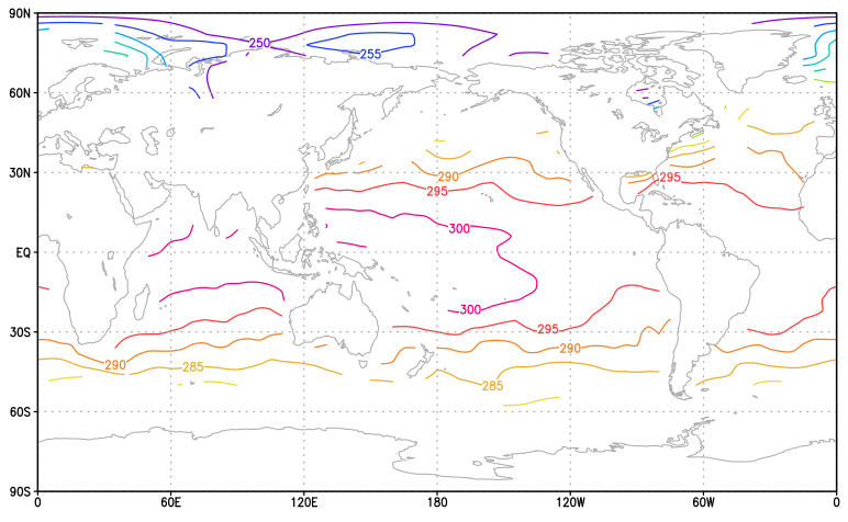
図10. 1000hPaの気温の空間分布


ga -> c
# 100hPaの気温の空間分布を描く。
ga -> set lev 100
ga -> d tair

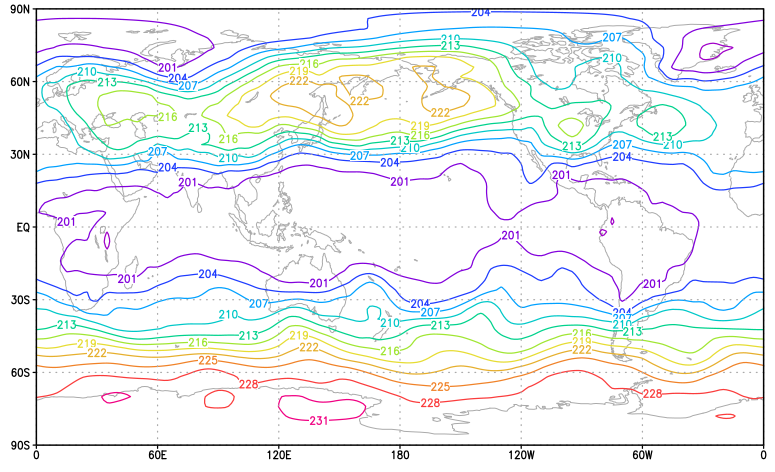
図11. 100hPaの気温の空間分布


ga -> c
# 気温の鉛直断面を描く。
ga -> set lon 180
LON set to 180 180
ga -> set z 1 7
LEV set to 1000 100
ga -> d tair

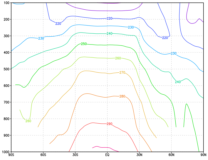
図12. 気温の鉛直断面

NetCDF形式のSSTデータを読む

NetCDF形式のERSSTデータの2000年1月の分布図を描画する。


$ grads

Grid Analysis and Display System (GrADS) Version 2.2.1
Copyright (C) 1988-2018 by George Mason University
GrADS comes with ABSOLUTELY NO WARRANTY
See file COPYRIGHT for more information

Config: v2.2.1 little-endian readline grib2 netcdf hdf4-sds hdf5 opendap-grids,stn geotiff shapefile
Issue 'q config' and 'q gxconfig' commands for more detailed configuration information
Landscape mode? ('n' for portrait):
GX Package Initialization: Size = 11 8.5
ga-> sdfopen sst.mnmean.nc
Scanning self-describing file:  sst.mnmean.nc
SDF file sst.mnmean.nc is open as file 1
LON set to 0 360
LAT set to -88 88
LEV set to 0 0
Time values set: 1854:1:1:0 1854:1:1:0
E set to 1 1
ga-> set time 1jan2000
Time values set: 2000:1:1:0 2000:1:1:0
ga-> d sst
Contouring: -0 to 30 interval 3

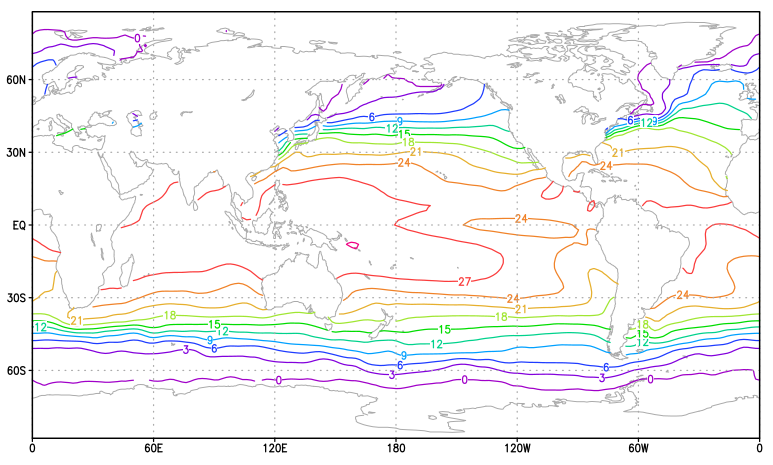
図13. 2000年1月の海面水温分布図

GRIB1形式のJRA-55データをGrADSで読む

“anl_surf125.202201”というファイルの中味を確認する。
まず、wgrib用のパラメータテーブルの環境変数GRIBTABをエクスポートする。


$ export GRIBTAB=./JRA55_anl_surf_ptable_wgrib.txt

wgribを用いてファイルの一番初めのデータの情報を得る.オプションの”-d 1”は最初のデータという意味。


$ wgrib -V -d 1 anl_surf125.202201

rec 1:0:date 2022010100 pres kpds5=1 kpds6=1 kpds7=0 levels=(0,0) grid=255 sfc anl:ave@6hr:
  pres="surface pressure [Pa]"
  timerange 123 P1 0 P2 6 TimeU 1  nx 288 ny 145 GDS grid 0 num_in_ave 124 missing 0
  center 34 subcenter 241 process 201 Table 200 scan: WE:NS winds(N/S)
  latlon: lat  90.000000 to -90.000000 by 1.250000  nxny 41760
          long 0.000000 to -1.250000 by 1.250000, (288 x 145) scan 0 mode 128 bdsgrid 1
  min/max data 51808.9 102921  num bits 12  BDS_Ref 518.089  DecScale -2 BinScale -3

ファイルに格納されている最初のデータは気圧”pres”であり、気象庁の番号表”Table 200”を使用し、緯度・経度の範囲と格子数、データの最小値と最大値、圧縮に関する情報が表示される。

次に、grib2ctl.plを用いてコントロールファイルを作成する。grib2ctl.plも環境変数GRIBTABを参照する。


$ grib2ctl.pl anl_surf125.202201 > anl_surf125.202201.ctl

作成されたコントロールファイルの中味は以下のようになっている。


dset ^./anl_surf125.202201
index ^./anl_surf125.202201.idx
undef 9.999E+20
title ./anl_surf125.202201
*  produced by grib2ctl v0.9.15
* command line options: ./anl_surf125.202201
dtype grib 255
options yrev
ydef 145 linear -90.000000 1.25
xdef 288 linear 0.000000 1.250000
tdef 1 linear 00Z01jan2022 1mo
zdef 1 linear 1 1
vars 9
airt2m  0 11,105,2 ** 2 m above ground "air temperature [K]"
depr2m  0 18,105,2 ** 2 m above ground "dewpoint depression [K]"
mslmsl  0 2,102,0 ** mean-sea level "mean sea level pressure [Pa]"
pottsfc  0 13,1,0  ** surface "potential temperature [K]"
pressfc  0 1,1,0  ** surface "surface pressure [Pa]"
rhum2m  0 52,105,2 ** 2 m above ground "relative humidity [%]"
sphum2m  0 51,105,2 ** 2 m above ground "speciphic humidity [kg/kg]"
uwnd10m  0 33,105,10 ** 10 m above ground "eastward wind [m/s]"
vwnd10m  0 34,105,10 ** 10 m above ground "northward wind [m/s]"
ENDVARS

“pressfc”の行をみると、変数名の右の最初の数字は鉛直の層数を示すが、ここでは”0”になっている。これはanl_surf125が地表面という1層だけのデータなのでこのようになっている。
その右の”1,1,0”はwgribの結果のkpds5 / kpds6 / kpds7にあたる。 kpds5が変数の数字符号であり、kpds6は鉛直層の種類、kpds7は鉛直層の高度を表している。

gribmapを用いてインデックスファイルを作成する。


$ gribmap -i anl_surf125.202201.ctl
gribmap: opening GRIB file anl_surf125.202201
gribmap: reached end of files
gribmap: writing the GRIB1 index file (version 5)

$ ls
anl_surf125.202201  anl_surf125.202201.ctl  anl_surf125.202201.idx

$ grads
ga-> open anl_surf125.202201.ctl
Scanning description file:  anl_surf125.202201.ctl
Data file ./anl_surf125.202201 is open as file 1
LON set to 0 360
LAT set to -90 90
LEV set to 1 1
Time values set: 2022:1:1:0 2022:1:1:0
E set to 1 1
# 海面更正気圧を描く
ga -> d mslmsl

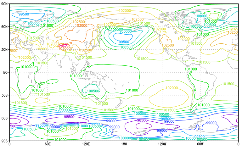
図14. 海面更正気圧の空間分布

NCL

米国NCARで開発された“NCAR Command Language”
Fortranに似たスクリプト言語である。ただし、次元の並びはC言語と同じである。Fortranでa(lon,lat,lev,time)とした場合、NCLではa(time,lev,lat,lon)となる。
NCLをインストールすると多くのスクリプトが利用可能である。また既存のFortranで書かれたサブルーチンをWRAPITすることにより、NCLで利用することができる。
大量の解析や作図の事例集が公開されている。
GrADSに比べるとnetCDF/GRIB/HDF等のファイルの取り扱いに制限が少ない。
【参考】東京大学先端科学技術研究センターの関澤氏が公開されている「NCL tips」

NetCDFファイルの読み方


$ conda activate ncl_stable
$ ncl
# ERSSTデータを読み込む準備。
ncl 0> fin = addfile("sst.mnmean.nc","r")
# 時刻データを読み込む。
ncl 1> time = fin->time
ncl 2> printVarSummary(time)

Variable: time
Type: double
Total Size: 16208 bytes
            2026 values
Number of Dimensions: 1
Dimensions and sizes:   [time | 2026]
Coordinates:
            time: [19723..81357]
Number Of Attributes: 8
  units :       days since 1800-1-1 00:00:00
  long_name :   Time
  delta_t :     0000-01-00 00:00:00
  avg_period :  0000-01-00 00:00:00
  prev_avg_period :     0000-00-07 00:00:00
  standard_name :       time
  axis :        T
  actual_range :        ( 19723, 81357 )

# cd_calendar()を用いてYYYYMMのフォーマットで時刻を確認。
ncl 3> print(cd_calendar(time,-1))
Variable: unnamed (return)
Type: integer
Total Size: 8104 bytes
            2026 values
Number of Dimensions: 1
Dimensions and sizes:   [2026]
Coordinates:
Number Of Attributes: 1
  calendar :    standard
(0)     185401
(1)     185402
(2)     185403
(3)     185404
(4)     185405
(5)     185406
(6)     185407
(7)     185408
(8)     185409
(9)     185410
(10)    185411
(11)    185412
(12)    185501
<<以下省略>>
# 1854年1月から毎月の時刻が格納されている。

# 1855年1月のSST（インデックス＝12が1855年01月）を読み込む
ncl 6> sst = fin->sst(12,:,:)
ncl 7> printVarSummary(sst)

Variable: sst
Type: float
Total Size: 64080 bytes
            16020 values
Number of Dimensions: 2
Dimensions and sizes:   [lat | 89] x [lon | 180]
Coordinates:
            lat: [88..-88]
            lon: [ 0..358]
Number Of Attributes: 12
  time :        20088
  long_name :   Monthly Means of Sea Surface Temperature
  units :       degC
  var_desc :    Sea Surface Temperature
  level_desc :  Surface
  statistic :   Mean
  missing_value :       -9.96921e+36
  dataset :     NOAA Extended Reconstructed SST V5
  parent_stat : Individual Values
  actual_range :        ( -1.8, 42.32636 )
  valid_range : ( -1.8, 45 )
  _FillValue :  -9.96921e+36

# ある月だけのデータを読み込んだため、sst の次元は [lat | 89] x [lon | 180] の
# 2次元になっている。このデータの空間分布図を作成してみる。

ncl 8> wks = gsn_open_wks("x11","test")
ncl 9> plot = gsn_csm_contour_map(wks, sst, False)
ncl 10> quit

$ conda deactivate

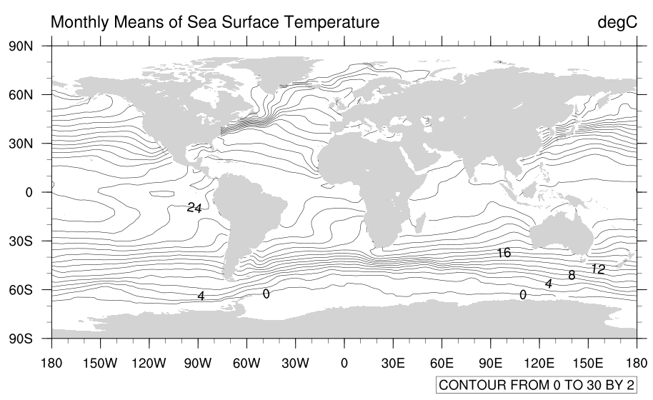
図15. ERSSTの1855年1月の海面水温分布図

左上の変数名はsstの属性”long_name”が反映されており、右上の単位はsstの属性”units”が反映されている。

JRA-55の読み方

パラメータテーブルを作成し、環境変数NCL_GRIB_PTABLE_PATHをエクスポートする。


$ less JRA55_anl_surf_ptable_ncl.txt
-1:34:241:200
1 : pres : Pa : surface pressure
2 : msl  : Pa : mean sea level pressure
11 : airt : K : air temperature
13 : pott : K : potential temperature
18 : depr : K : dewpoint depression
51 : sphum : kg/kg : speciphic humidity
52 : rhum : % : relative humidity
33 : uwnd : m/s : eastward wind
34 : vwnd : m/s : northward wind

$ export NCL_GRIB_PTABLE_PATH=./JRA55_anl_surf_ptable_ncl.txt

condaの仮想環境”ncl_stable”をアクティベートする。


$ conda activate ncl_stable
$ ncl
Copyright (C) 1995-2019 - All Rights Reserved
 University Corporation for Atmospheric Research
 NCAR Command Language Version 6.6.2
 The use of this software is governed by a License Agreement.
 See http://www.ncl.ucar.edu/ for more details.
ncl 0> fin = addfile(“anl_surf125.202201”,”r”)

“.grib”と拡張子が付けられている場合はGRIBと判断すると公式webサイトに記述があるが、“.grib”という拡張子なしでも読めている。しかし、確実にGRIBとしてファイルを読むためには


ln -s anl_surf125.202201 anl_surf125.202201.grib

として、シンボリックリンクを張ればよい。


# ファイルに格納されている変数等の情報を確認する。
ncl 1> print(fin)
Variable: fin
Type: file
filename:       anl_surf125.202201
path:   anl_surf125.202201
   file global attributes:
   dimensions:
      g0_lat_0 = 145
      g0_lon_1 = 288
   variables:
      float pres_GDS0_SFC_S123 ( g0_lat_0, g0_lon_1 )
         sub_center :   241
         center :       Japanese Meteorological Agency - Tokyo (RSMC)
         long_name :    surface pressure
         units :        Pa
         _FillValue :   1e+20
         level_indicator :      1
         gds_grid_type :        0
         parameter_table_version :      200
         parameter_number :     1
         forecast_time :        0
         forecast_time_units :  hours
         initial_time : 01/01/2022 (00:00)
         statistical_process_descriptor :       average of N uninitialized analyses
         statistical_process_duration : instantaneous (beginning at reference time at intervals of 6 hours)
         N :    124

      float msl_GDS0_MSL_S123 ( g0_lat_0, g0_lon_1 )
         sub_center :   241
    << 以下省略 >>

# 気圧のデータを読み込む。
ncl 2> pres = fin->pres_GDS0_SFC_S123
# 読み込んだ気圧の情報を確認する。
ncl 3> printVarSummary(pres)

Variable: pres
Type: float
Total Size: 167040 bytes
            41760 values
Number of Dimensions: 2
Dimensions and sizes:   [g0_lat_0 | 145] x [g0_lon_1 | 288]
Coordinates:
            g0_lat_0: [90..-90]
            g0_lon_1: [ 0..358.75]
Number Of Attributes: 15
  sub_center :  241
  center :      Japanese Meteorological Agency - Tokyo (RSMC)
  long_name :   surface pressure
  units :       Pa
  _FillValue :  1e+20
  level_indicator :     1
  gds_grid_type :       0
  parameter_table_version :     200
  parameter_number :    1
  forecast_time :       0
  forecast_time_units : hours
  initial_time :        01/01/2022 (00:00)
  statistical_process_descriptor :      average of N uninitialized analyses
  statistical_process_duration :        instantaneous (beginning at reference time at intervals of 6 hours)
  N :   124
ncl 4> quit

$ conda deactivate

GrADS形式バイナリファイルの読み方


$ ncl
# GrADSのチュートリアルに使われるサンプルデータを読んでみる。
# model.dat は little endian で書き出されているので、オプションを設定する。
ncl 0> setfileoption("bin","ReadByteOrder","LittleEndian")

# 経度方向に72格子、緯度方向に46格子なので、次元の大きさを指定する。
ncl 1> dims = (/46,72/)

# 最初のデータ（インデックス＝0）を読み込むため nrec を指定する。
ncl 2> nrec = 0

# 最初のデータを読み込む。
ncl 3> x = fbindirread("model.dat", nrec, dims, "float")

# xがどのようなものか確認。
ncl 4> printVarSummary(x)
Variable: x
Type: float
Total Size: 13248 bytes
            3312 values
Number of Dimensions: 2
Dimensions and sizes:   [46] x [72]
Coordinates:

# “Coordinates”がないので、緯度・経度を作成して付与する。
# model.ctlの記述からlat/lonを作成する。
ncl 5> lat=-90.0+ispan(0,45,1)*4.0
ncl 6> lat!0 = "lat"
ncl 7> lat&lat = lat
ncl 8> lat@units = "degrees_north"
ncl 9> lon = 0.0 + ispan(0,71,1)*5.0
ncl 10> lon!0     = "lon"
ncl 11> lon&lon   =  lon
ncl 12> lon@units = "degrees_east"

# 作成した緯度・経度をxに付与する。
ncl 13> x!0 = "lat"
ncl 14> x!1 = "lon"
ncl 15> x&lat = lat
ncl 16> x&lon = lon

# model.datの最初のデータは地上気圧なので、long_name、units、_FillValue、
# missing_valueをmodel.ctlを見ながら付与する。
ncl 17> x@long_name = "Surface Pressure"
ncl 18> x@units = "hPa"
ncl 19> x@_FillValue = -2.56E33
ncl 20> x@missing_value = -2.56E33

# 変数xの情報を確認する。
ncl 21> printVarSummary(x)
Variable: x
Type: float
Total Size: 13248 bytes
            3312 values
Number of Dimensions: 2
Dimensions and sizes:   [lat | 46] x [lon | 72]
Coordinates:
            lat: [-90..90]
            lon: [ 0..355]
Number Of Attributes: 4
  missing_value :       -2.56e+33
  _FillValue :  -2.56e+33
  units :       hPa
  long_name :   Surface Pressure

ncl 22> wks = gsn_open_wks("x11","test")
ncl 23> plot = gsn_csm_contour_map(wks, x, False)
ncl 24> quit

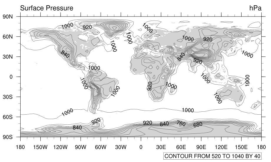
図16. model.datの地上気圧データ

地上気圧の空間分布が描かれた。左上の”Surface Pressure”は気圧の属性x@long_name、右上の”hPa”は気圧の属性x@unitsが反映されている。

d4PDF_RCMの可視化

d4PDF_RCMのtopo_essp20.datを用意する。NCLを用いてtopo_essp20.datをNetCDF形式に変換する。topo_essp20.datはFortranでsequential accessで出力されているので、スクリプトの中でfbinrecreadを用いる。“;”以降はコメント。


$ less proc01.ncl
begin
nameIn="topo_essp20.dat"
setfileoption("bin","ReadByteOrder","BigEndian")
dims = (/155,191/)
lat2d = fbinrecread(nameIn,0,dims,"float")
lon2d = fbinrecread(nameIn,1,dims,"float")
alt   = fbinrecread(nameIn,2,dims,"float")
land  = fbinrecread(nameIn,3,dims,"float")

lat = ispan(0,154,1)*0.1 ;; 仮の緯度。ダミー
lat!0 = "lat"
lat&lat = lat
lat@units = "degrees_north"

lon = ispan(0,190,1)*0.1 ;; 仮の経度。ダミー
lon!0 = "lon"
lon&lon = lon
lon@units = "degrees_east"

lat2d!0 = "lat"
lat2d!1 = "lon"
lat2d&lat = lat
lat2d&lon = lon
lat2d@units = "degrees_north"
lat2d@long_name = "latitude"

lon2d!0 = "lat"
lon2d!1 = "lon"
lon2d&lat = lat
lon2d&lon = lon
lon2d@units = "degrees_east"
lon2d@long_name = "longitude"

alt!0 = "lat"
alt!1 = "lon"
alt&lat = lat
alt&lon = lon
alt@units = "m"
alt@long_name = "surface elevation"

land!0 = "lat"
land!1 = "lon"
land&lat = lat
land&lon = lon
land@units = "none"
land@long_name = "land sea fraction"

fout = addfile("topo_essp20.nc","c")
fAtt = True
fAtt@title = "d4PDF_RCM. Topography, Lans-sea fraction, latitude, longitude data"
fAtt@source_file = "topo_essp20.dat / topo_essp20.ctl"
fAtt@Conventions = "None"
fileattdef( fout, fAtt )
fout->alt = alt
fout->land = land
fout->lat2d = lat2d
fout->lon2d = lon2d
end

$ ncl ./proc01.ncl
$ ncdump -h topo_essp20.nc
netcdf topo_essp20 {
dimensions:
        lat = 155 ;
        lon = 191 ;
variables:
        float alt(lat, lon) ;
                alt:long_name = "surface elevation" ;
                alt:units = "m" ;
        float lat(lat) ;
                lat:units = "degrees_north" ;
        float lon(lon) ;
                lon:units = "degrees_east" ;
        float land(lat, lon) ;
                land:long_name = "land sea fraction" ;
                land:units = "none" ;
        float lat2d(lat, lon) ;
                lat2d:long_name = "latitude" ;
                lat2d:units = "degrees_north" ;
        float lon2d(lat, lon) ;
                lon2d:long_name = "longitude" ;
                lon2d:units = "degrees_east" ;
// global attributes:
                :Conventions = "None" ;
                :source_file = "topo_essp20.dat / topo_essp20.ctl" ;
                :title = "d4PDF_RCM. Topography, Lans-sea fraction, latitude, longitude data" ;
}
# 変数lat2dは各格子の緯度の値を保持し、変数lon2dは各格子の経度の値を保持している。
$ ncview topo_essp20.nc

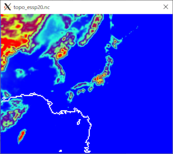
図17. d4PDF_RCMの標高分布

図中の白い線は、緯度・経度がダミーなため描かれてしまったものなので無視すること。

surf_HPB_m001_200001.gribから気温のデータを1タイムステップだけ切り出す。


$ wgrib surf_HPB_m001_200001.grib -d 11 -grib -o test.1.grib
11:474510:d=00010101:TMP:kpds5=11:kpds6=1:kpds7=0:TR=0:P1=0:P2=0:TimeU=2:sfc:anl:NAve=0

NCLを用いた可視化ではtopo_essp20.ncに格納されているlon2dとlat2dを読み込み、作図したい変数の属性として付与する必要がある。
なお、NCL のスクリプト内部では“;”以降はコメントである。


$ less mkfig1.ncl
begin
fin1 = addfile("test.1.grib","r") ;; 
airt = fin1->TMP_GDS0_SFC ;;気温データを読み込む

fin2 = addfile("topo_essp20.nc","r")
lat2d = fin2->lat2d ;; 緯度情報のデータを読み込む
lon2d = fin2->lon2d ;; 経度情報のデータを読み込む

;; airtの属性としてlat2d/lon2dを付与する。
airt@lat2d = lat2d
airt@lon2d = lon2d

wks = gsn_open_wks("x11","fig1")
res = True
res@gsnMaximize = True
res@mpLambertParallel1F = 30.0 ;; ランベルト正角円錐図法の基準緯度1
res@mpLambertParalle12F = 60.0 ;; ランベルト正角円錐図法の基準緯度2
res@mpLambertMeridianF  = 135.0 ;; ランベルト正角円錐図法の基準経度

res@mpLimitMode         = "Corners"
res@mpLeftCornerLatF    = 15.0
res@mpLeftCornerLonF    = 105.0
res@mpRightCornerLatF   = 52.0
res@mpRightCornerLonF   = 165.0
res@mpDataBaseVersion   = "MediumRes"
res@pmTickMarkDisplayMode = "Always"
res@cnFillOn  = True
res@cnLinesOn = False
plot = gsn_csm_contour_map(wks, airt, res)
end

$
$ ncl ./mkfig1.ncl

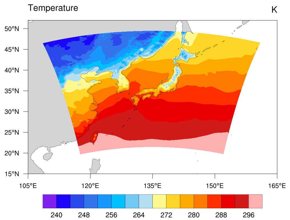
図18. NCLでd4PDF_RCMの気温分布を描画

NCLを用いたd4PDF_RCMのデータ処理では、

x方向191格子、y方向に155格子の単純なマトリックス（配列）としてデータを見て、同一格子上での変数間の四則演算や、時間方向の処理を行う。ただし緯度や経度を考慮しなくてもよい処理のみ。
空間的な処理を行う（例えば緯度や経度を考慮すべき処理や内挿処理）、または可視化するときには、topo_esssp20.datに格納されている緯度と経度の情報を読み込んで処理をする。

という手順が現実的である。

ところで、GrADSを用いたd4PDF_RCMの可視化はd4PDF_RCMの一部として配布しているコントロールファイルを用いれば簡単にできる。


$ less surf_HPB_m001_200001.ctl
***output grads ctl file for surf***
dset surf_HPB_m001_200001.grib
index surf_HPB_m001_200001.idx
pdef 191 155 LCCR 35 135 97 77 30 60 135 20000 20000
dtype grib 255
undef -9.9999e+20
<<以下省略>>

GrADSの場合はコントロールファイルのpdefの行が重要である。この行の意味は、x方向に191格子、y方向に155格子、ランベルト正角円錐図法で風の成分の方向転換済み(LCCR)、データのある一点の緯度・経度(35N,135E)と対応する格子のインデックス番号(97,77)、投影法の基準緯度二つ(30N, 60N)、投影法の基準経度(135E)、格子のx方向の間隔(20000m)、格子のy方向の間隔(20000m)となっている。 GrADSはこの情報を利用して、データを地図上に描いてゆく。

現実的には解析担当者が意識をせず、通常通りにコントロールファイルを開いて、’d tmp’とすれば可視化が実行される。


ga -> open surf_HPB_m001_200001.ctl
<<以下省略>>
ga -> d tmp

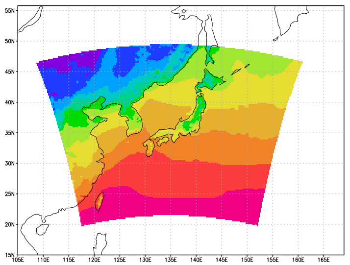
図19. GrADSでd4PDF_RCMの気温分布を描画

【参考】Python

Python言語は、習得することはそれほど難しくないとされる言語である。まずは、numpy、scipy、pandas、matplotlibの使い方を覚えると良い。そしてPythonは、急速に様々なパッケージ（ライブラリ）開発が進んでいる言語であるため、あるパッケージがほかのどのパッケージに依存しているのかなど、自分で調査して試してみる必要がある。なにか問題が生じた場合、パッケージがGitHubを使用しているのならばissueは要チェックであり、stackoverflowでの投稿などを検索することも必要となる。そして情報の多くは英語であるため、気候データ処理の初心者がPythonを使用することは少しハードルが高いかもしれない。だが、今後は気候学のデータ処理の中心はPythonに移行することは明確なので（米国UCAR/NCARが今後はNCLの開発は停止して、PythonのライブラリGeoCATの整備に注力することを宣言済み）、頑張って使い方を覚えると、先々良いことがあると思われる。

netcdf4-python
NetCDFライブラリを作成したUnidata作成のNetCDF読み書き用パッケージ。
Iris
英国気象局などが開発中の気候データ読み書き・作図パッケージ。
xarray
現在活発に開発が続いている多次元データを取り扱うパッケージ。
PyNIO/PyNGL
UCARで開発されていたNetCDF等の読み書きパッケージとNCLから移植した作図パッケージ。 UCARでは新たなPythonをベースとしたパッケージ群を開発中で、その一部が GeoCATである。
【参考】国立環境研究所の山下氏が公開されている
「気象データ解析のためのmatplotlibの使い方」。

【参考】統計解析向けのプログラミング言語：R言語

R言語には地理情報関係のパッケージ群が存在する。それらのパッケージ群を使用して観測地点に最も近い領域気候モデルのグリッドポイントを検索する例を示す。

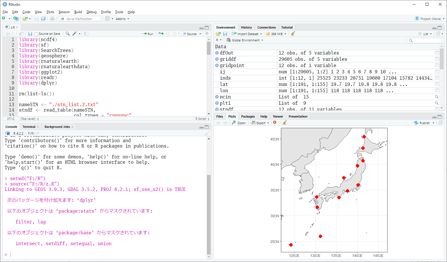
図20. Rstudioの画面

左上のペインはスクリプトファイルの編集画面になっている。
左下のペインはRのコマンドを実行するコンソール画面となっている。
右上のペインは変数やオブジェクトの情報や、コンソールで実行したコマンドの履歴などの情報が得られるようになっている。
右下のペインは作成した図を表示する画面やパッケージの管理画面にもなっている。

今回紹介する例の実行に必要なパッケージを、左下のコンソールで"install.packages()"関数を用いてインストールする。例えば"ncdf4"をインストールするには、以下のようにする。


> install.packages(“ncdf4”)

インストールするパッケージ：

パッケージ	内容
readr	ファイルを読むためのパッケージ
dplyr	データフレームを処理するためのパッケージ
ggplot2	作図に用いるパッケージ
ncdf4	NetCDFを読み書きするためのパッケージ
sf	地理情報関係のパッケージ
geosphere	球面上の距離や角度を計算するパッケージ
rnaturalearth	地図データのパッケージ
rnaturalearthdata	地図データのパッケージ
SearchTrees	ツリー構造のデータの検索パッケージ

国内のラジオゾンデ観測地点の地点番号、緯度、経度、標高、地点名のリストを用意する。なお、緯度・経度は度と分に分かれている。


$ less ./stn_list.2.txt
47401 45 24.9 141 40.7   12  Wakkanai
47412 43 03.6 141 19.7   17  Sapporo
47580 40 42.0 141 22.0   39  Misawa
47582 39 43.1 140 06.0    6  Akita
47600 37 23.5 136 53.7    5  Wajima
47646 36 03.5 140 07.5   25  Tateno
47681 34 45   137 42     47  Hamamatsu
47778 33 27.1 135 45.7   73  Shionomisaki
47807 33 35.0 130 23.0   12  Fukuoka
47827 31 33.3 130 32.9   31  Kagoshima
47918 24 20.2 124 09.8    6  Ishigakijima

以下のスクリプトを適当な名前を付けて保存する。ただし、”#”で始まる行は除く。
なおこのスクリプトはtidyverseな仕様なので “%>%” というあまり見慣れない演算子があらわれるが、そのまま打ち込むこと。


library(SearchTrees)
library(ncdf4)
library(sf)
library(geosphere)
library(rnaturalearth)
library(rnaturalearthdata)
library(ggplot2)
library(readr)
library(dplyr)

rm(list=ls())

nameSTN <- "./stn_list.2.txt"
stndf <- read_table(nameSTN,
                    col_types = "cnnnnnc",
                    col_names = c("StnIdx","latD","latM","lonD","lonM",
                                  "height","StnName"))

# 緯度・経度を度分から度に直して、mutateする。
# sfオブジェクトにする際に緯度・経度が別に必要となるので、mutateする。
stndf <- stndf %>%
  mutate(lon = lonD + lonM / 60.0, lat = latD + latM / 60.0) %>%
  mutate(lonX = lon, latY = lat)

# sfオブジェクトに変換する。それぞれのデータ（行）にgeometryが付加される。
# また日本測地系2000における地理座標系(JGD2000, EPSG=4612)を利用する。
stndf2<- st_as_sf(stndf, coords = c("lonX", "latY"), crs = 4612)

# 領域気候モデルd4PDF_RCMの緯度と経度のデータを読む。
nameTopo <- "./topo_essp20.nc"
ncin <- nc_open(nameTopo)
lat <- ncvar_get(ncin, "lat2d")
lon <- ncvar_get(ncin, "lon2d")

# 2次元データであるlat / lon をベクトルに変換する。
lonX <- as.vector(lon)
latY <- as.vector(lat)

# モデルのx方向とy方向の格子数から各格子の格子番号を作成する。
nlat <- 155
nlon <- 191
ii <- seq(1, nlon, 1)
jj <- seq(1, nlat, 1)
ij <- as.matrix(expand.grid(ii, jj))

# モデルの格子情報をデータフレームにする。
tmp_df <- data.frame(cbind(ij, lonX, latY, lonX, latY))
colnames(tmp_df) <- c("ii","jj","lon","lat","lonX","latY")

# 以下のようなデータフレームを作った。
#   ii jj      lon      lat     lonX     latY
# 1  1  1 117.5693 19.67914 117.5693 19.67914
# 2  2  1 117.7452 19.71560 117.7452 19.71560
# 3  3  1 117.9214 19.75170 117.9214 19.75170

# sfオブジェクトに変換する。sfオブジェクトに変換するとplot()が利用できる。
griddf<- st_as_sf(tmp_df, coords = c("lonX", "latY"), crs = 4612)

# griddf は以下のような構造。
# 各行（＝各格子点）にgeometryが付加された。
# Simple feature collection with 6 features and 4 fields
# Geometry type: POINT
# Dimension:     XY
# Bounding box:  xmin: 117.5693 ymin: 19.67914 xmax: 118.4508 ymax: 19.85786
# Geodetic CRS:  JGD2000
#   ii jj      lon      lat                  geometry
# 1  1  1 117.5693 19.67914  POINT (117.5693 19.67914)
# 2  2  1 117.7452 19.71560  POINT (117.7452 19.7156)
# 3  3  1 117.9214 19.75170  POINT (117.9214 19.7517)

# griddfをプロット。
plot(griddf)
# スクリプトは後に続く

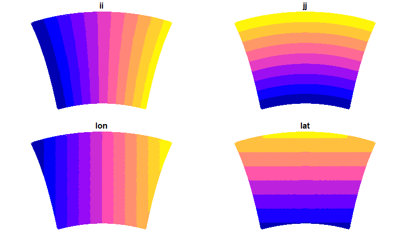
図21. griddfの表示

x方向のインデックスiiも、y方向のインデックスjjもカーブをもった分布をしている。一方で経度lonは縦方向で、緯度latは横方向できれいにそろっている。つまり正しくデータがsfオブジェクトに格納されたことを意味している。

スクリプトの続き。


# 各格子点の緯度・経度の値からツリー構造のデータを作成する。
# なおこの時点では、座標系などを考慮しない単なる数字の羅列になってしまう。
tree <- createTree( st_coordinates( griddf ) )

# 各ラジオゾンデ観測地点の緯度・経度を “newx” / “newy” に代入して、
# 一番近い格子点を探す（k=1）。
# ”inds”には格子点のインデックス(griddfの行番号)が返される。
# 行番号とはgriddfの構造を見たときの一番左側の数字のこと。
inds <- knnLookup( tree, newx = stndf2$lon, newy = stndf2$lat, k = 1 )

# 各ラジオゾンデ観測地点にもっとも近いモデル格子点の情報をデータフレームにする。
x <- griddf[inds,]$lon
y <- griddf[inds,]$lat
ii2 <- griddf[inds,]$ii
jj2 <- griddf[inds,]$jj
dfOut <- data.frame(StnIdx=stndf$StnIdx, ii=ii2, jj=jj2, lon=x, lat=y)

# 得られた結果を csv ファイルに保存する。
write.csv(dfOut, "./nhrcm_raob.csv", row.names = FALSE)

# 出力は以下の様な形をしている。ii はx方向の格子番号、jjはy方向の格子番号
# "StnIdx","ii","jj","lon","lat"
# "47401",122,134,141.635116577148,45.3641014099121
# "47412",122,122,141.3818359375,43.1371574401855

# 検索したグリッドがラジオゾンデ観測地点に本当に近いのか図にして確認。
gridpoint <- st_as_sf(data.frame(lon=x, lat=y), coords=c("lon","lat"), crs = 4612)
world <- ne_countries(scale = 'medium', returnclass = 'sf')
plt1 <- ggplot() + geom_sf(data = world) +
  geom_sf(data = gridpoint, shape = 16, size = 4, color = "red") +
  coord_sf(xlim = c(123,146), ylim = c(24,46)) + theme_bw()
plot(plt1)

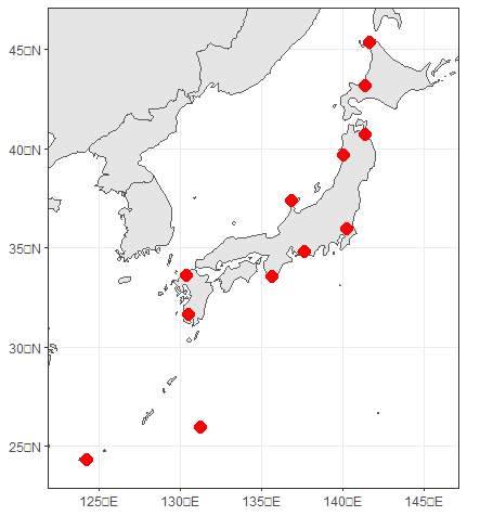
図22. ラジオゾンデ観測点に最も近いグリッドの分布図

47401（稚内）の経度は141.6783、緯度は45.415なので、観測点ともっとも近いモデルのグリッドは、経度方向で0.043度、緯度方向で0.05度離れている。例えば geosphere::distVincentySphere() で距離を計算すると約6.6km離れている。
knnLookup()で”k=3”とすると、観測点近傍の3グリッドの情報が返ってくる。この情報を利用し、geosphereの距離計算関数を用いて観測点と気候モデルのグリッドの距離を比較して、計算結果が正しいのかを確認してもよい。
稚内にもっとも近いグリッドのデータをd4PDF_RCMのファイルから取り出すには、x方向のインデックスii、y方向のインデックスjjである位置にある値を選択すればよい。
なお、気候モデルは地球を楕円体として取り扱っていないので、あまり厳密な比較は避けるべきである。

TOOL ツール紹介

TOOL DS2022気候予測データのファイル・フォーマットとツール類の紹介 令和6年3月

はじめに

免責事項

前書き

DS2022気候予測データの主要なファイル・フォーマット

GRIB / GRIB2

NetCDF

いわゆる「GrADS形式」

サンプルデータ

NOAA Extended Reconstructed SST V5

気象庁55年長期再解析(JRA-55)

d4PDF_RCM

GrADSのexampleデータ

データ・ビューアー

ncview

Panoply

wgrib / wgrib2

パラメータテーブル

ファイルの確認

データの抽出

Climate Data Operators (cdo)

パラメータテーブル

ファイルの確認

GRIB1形式からNetCDF形式への変換

GrADS用バイナリファイルからNetCDF形式への変換

指定した変数の抽出

指定した年のデータの抽出

ファイルの結合

指定した領域のデータの切り出し

統計値の作成

GrADS

GrADS用バイナリファイルmodel.datを読む

NetCDF形式のSSTデータを読む

GRIB1形式のJRA-55データをGrADSで読む

NCL

NetCDFファイルの読み方

JRA-55の読み方

GrADS形式バイナリファイルの読み方

d4PDF_RCMの可視化

【参考】Python

【参考】統計解析向けのプログラミング言語：R言語

TOOL
ツール紹介

TOOL DS2022気候予測データの
ファイル・フォーマットとツール類の紹介
令和6年3月